Set a cup of hot tea on the table. The tea starts out hot but cools off. Now set a glass of iced tea next to the cup of cooling hot tea; the iced tea will warm up. If we wait long enough, both teas would settle at the temperature of the room. What's going on with the tea? How could we model this? How can we explain it?

We could try to model this behavior by looking for functions that we know exhibit the expected behavior (start high, then decrease until a certain level), but that rings a bit false, and it won't have much explanatory power. Instead, we'd like to write down a mathematical description of the physical phenomena at play, and use that description to understand the behavior of the cooling and warming teas.

One thing we need to deal with is: unlike interest, which happens discretely in time (every so often), the tea is continuously cooling.

The Mathematical Model

We will track the rate of change of temperature of the tea. What would it depend on? If we brainstorm, we generate a few ideas:

The bigger the temperature difference between the drink and the air, the faster temperature will change. That is, very hot things cool off faster than moderately hot things.
The smaller the cup, the faster the temperature will change. A big pot of soup could take hours to cool off.
The material of the cup matters: tea in a metal cup would cool off faster than tea in a styrofoam cup, because metal conducts heat very well and styrofoam conducts heat poorly. Tea in a double-wall insulated ceramic mug will cool very slowly.
A cup in the wind will cool off faster than a cup in still air.
In the iced-tea case, the ice melting will have an effect on the rate at which the tea warms up. What kind of ice is it? One big cube, or crushed ice?

There are so many factors we could include, but let's start simple, and implement the first assumption in a simple way: the rate at which temperature of the drink changes is proportional to the difference between the temperature of the drink and the ambient temperature. By "is proportional to", we mean, is some multiple of.

screencast: deriving the mathematical model

Let's use the following symbols:

symbol	meaning	units
$t$	time	minutes
$y$	temperature of drink	°F
$R$	temperature of the room	°F
$K$	thermal conductivity constant	???

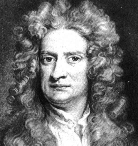
I'll explain what $K$ means in a moment. But first let's form our equation from the assumption the rate at which temperature of the drink changes is proportional to the difference between the temperature of the drink and the ambient temperature. (This is known as Newton's Law, after Isaac Newton.)

$\frac{dy}{dt}=K\cdot (y-R)$

The symbol $\frac{dy}{dt}$ , you'll recall, denotes the rate of change of $y$ . $K$ is which multiple of the difference between $y$ and $R$ . It's traditional to arrange things so that all the constants like $K$ are positive.

Whenever you convert an assumption or a word equation into a symbolic equation, you can do some sanity checks of your assumptions using the symbolic equation. Plug in a few values for the variables, ask about signs, things like that. If the result makes sense, that doesn't mean your model is definitely right -- but if the sanity check fails, it means one of two things: either your equation was improperly derived from the assumptions (most likely), or the assumptions themselves are not reasonable.

Let's check a few things to make sure our equation makes at least a little sense. First, what if the temperature of the drink is greater than the room temperature (symbolically, if $y>R$ )? We expect that the drink should start cooling off, that is, that $\frac{dy}{dt}<0$ . But since $y>R$ , $y-R>0$ , so we'd have $\frac{dy}{dt}=K(y-R)>0$ . Oops!

To fix this, let's replace our equation with

$\frac{dy}{dt}=K\cdot (R-y)$

That way, when $y>R$ , $\frac{dy}{dt}<0$ , which is as it should be.

What if we got lucky and brewed a perfectly room-temperature cup of tea, that is, if $y=R$ ? Then we'd expect the tea to just stay at room temperature, so $\frac{dy}{dt}=0$ . This is borne out by our equation, because if $y=R$ , then $K(R-y)=K(R-R)=0$ .

Notice we were able to deduce a lot about the behavior of the solutions of a differential equation (when they are constant, when they are increasing, when they are decreasing) without actually solving the equation. We just had to look at the equation itself. This is called "a priori" (Latin: 'from before', as in 'from before even finding a solution') reasoning about the equation.

Now, we'd like to solve the initial value problem

$\begin{cases} \frac{dy}{dt}=K(R-y)\\y(0)=y_0\end{cases}$

where $y_0$ is the initial temperature of the cup of tea. How to do this?

The Computational Methods

As usual, there are two broad approaches: analytical and numerical or approximate.

Analytical Solution (Maple)

Maple actually knows how to find explicit solutions to differential equations; that is, it will find a function $y(t)$ for us -- at least some of the time.

First, we should tell Maple about the equation we want to solve:

[> NewtsLaw:=diff(y(t),t)=K*(R-y(t));

which is just the Maple way of expressing $\frac{dy}{dt}=K(R-y)$ :

Maple now knows that $y$ is a function of $t$ , and it knows how to solve differential equations:

[> dsolve(NewtsLaw,y(t));

which tells us that $y(t)=R+Ce^{-Kt}$ for some constant $C$ , which will be determined by the initial temperature $y(0)$ .

We can also ask Maple to solve the initial value problem all at once:

[> dsolve({NewtsLaw,y(0)=y0},y(t));

Here the curly brackets { } tell Maple to solve a system of equations rather than just one equation.

Let's plug in a few specific values using the subs command and check to see if this answer looks right. We'll set room temperature at 70 degrees, initial tea temperature at 200 degrees (a little less than boiling) and $K=\frac{1}{15}$ :

which looks about like you'd expect: the tea cools off fast initially, and then slows down as the temperature gets closer to 70 degrees.

Now you try it with values of $R$ and $y_0$ appropriate to iced tea.

Approximate Method (Excel)

a video walkthrough of this

Sometimes Maple can give us a nice formula, but some differential equations are too gnarly for even Maple to sort out. What to do then? Excel, and Lessons 5 and 6, offer a kludgey sort of way to get around this.

The idea is to, instead of thinking of time as continuous, pretend that it's broken up into discrete chunks (say, minutes). Let's let $D$ be the duration of each time interval. Then instead of Newton's Law

$\frac{dy}{dt}=K(R-y)$

we can say something like: the new temperature (at time n+1) is the old temperature (at time n), plus an amount proportional to the difference between the old temperature and the ambient temperature, or in symbols,

$y_{n+1}=y_n+K\cdot D\cdot (R-y_n)$

where we've included the length of the time interval $D$ explicitly. (This is the right way to do things -- a larger $D$ will automatically result in more change between $y_{n+1}$ and $y_n$ .) We should also note the relationship the current time is the number of time intervals times the length of each time interval, or in symbols,

$t=n\cdot D$

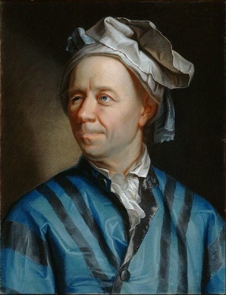
What we have is a finite difference model, which we can use Excel to numerically model (as we did in Lessons 5 and 6), by iteration. This approach is known as Euler's method, after Leonhard Euler, who worked long before Excel existed and had to do everything by hand.

First set up a sheet with columns for $t$ , our approximation of $y$ , the exact solution for $y$ that Maple found, and a percent error to compare them. To keep things loose, put some cells for our parameters off to the side:

(Here we've used the analytical solution in column C as our "actual" answer in the percent error formula because we believe it's "more correct" than the iterative column B.)
We'll say the initial temperature is 200 degrees, room temperature is 70, and $K=1/15$ as before; we'll populate column C with the Excelified version of the formula Maple gave us. Excel doesn't know about $e$ , so we have to write "EXP" for this function.

Note the $ in references to the cells containing 200, 1/15, and 70.
Let's say that we measure time in minutes, and take a time interval of 5 minutes. So $D=5$ . Then column A should be populated by the formula:

because we've added 5 to the previous time value.
Now, we use an Excelified version of the finite-difference model $y_{n+1}=y_{n}+K\cdot D\cdot (R-y_n)$ :
For the analytical solution, we can just copy-and-paste the formula from cell C2 into C3, and also copy-and-paste the percent error:
Since Excel is good at recognizing patterns, we can just highlight all the cells we want to extend (A3:D3), grab the lower right corner, and use it to drag down:

As we would expect, the temperature is predicted by both models to settle down around 70 degrees. It takes about 65 minutes until the tea is predicted by the iterative method to be within 1 degree of room temperature.

To enter a fraction in Excel, don't just type "1/15". Excel will think you mean January 15th. You need to tell Excel you mean the number, so you'll need to type "=1/15".

Analyzing the Approximate Method

Our choice of time interval was just that -- a choice we made. We could have chosen differently. What if we set $D=10$ ?

The values of the analytical model stay the same (since it doesn't depend on D), but the iterative method now says it only takes 50 minutes for the tea to be within 1 degree of room temperature. Also notice how much higher the errors are!

What if we take a smaller D? You play around with that.

Takeaways/Deliverables

To say you've successfully completed this lesson, you should be able to do the following:

Formulate a differential equation representing Newton's Law.
Use Maple's dsolve command to find an analytical solution to the differential equation
Use Excel to carry out Euler's method of approximating solutions to a differential equation.
Compare the result of Euler's method and the analytical solution.

These skills are what you'll need to complete the WebAssign homework for this Lesson.

I know which one of these dudes I'd invite to my house. (Hint: Not the one whose name rhymes with "shootin'".)